How does Lasso Regression (L1) Encourage Zero Coefficients but not L2?

We often read almost everywhere that Lasso regression encourages zero coefficient, and hence provides a great tool for variable selection as well but it is really difficult to get the intuition about this. In this article, I have tried to discuss this in detail.

Overfitting and Regularization
Intuition 1: Optimize a single coefficient model
Intuition 2: Look at this simple example
Intuition 3: Observe this beautiful image
Intuition 4: Probabilistic Interpretation of L1 and L2

Overfitting and Regularization

Overfitting is a phenomenon where a machine learning model is unable to generalize well on the unseen data. When our model is complex (for example polynomial regression with a very high degree or a very deep neural network) and we have less training data, in those cases model tends to memorize the training data and does not generalize well on unseen data.

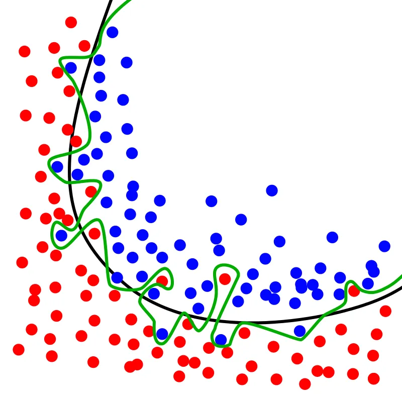
Figure 1: The green line represents an overfitted model and the black line represents a regularized model. While the green line best follows the training data, it is too dependent on that data and it is likely to have a higher error rate on new unseen data, compared to the black line. (Source: Wikipedia)

Look at this image from Wikipedia in which the green line shows the decision boundary of the overfitted classifier while the black one shows the regularized one. We see that even though the green decision boundary seems to give no training error it won't generalize well on the unseen data.

Regularization is one of the ways to reduce the overfitting of a machine learning model by adding the extra penalty to the loss function. The penalty is added in terms of some norms of the parameters. When the loss function of the linear regression model uses the L1 norm of the parameters, the regression model is called Lasso Regression while the one which uses the L2 norms is called Ridge Regression.

Intuition 1: Optimize a Single Coefficient Model

As explained here, consider a Ridge Regression model with a single coefficient β, the equation for the loss function of L2 regression in this can be given as follows:

$$\text{Loss}_{L2} = \sum_{i=1}^{n} (y_i - \beta x_i)^2 + \lambda \beta^2$$

To minimize this equation, we take the derivative w.r.t β and equate it to 0 to get the coefficient's optimal value:

$$\frac{\partial \text{Loss}_{L2}}{\partial \beta} = -2\sum_{i=1}^{n} x_i(y_i - \beta x_i) + 2\lambda\beta = 0$$ $$\beta = \frac{\sum_{i=1}^{n} x_i y_i}{\sum_{i=1}^{n} x_i^2 + \lambda}$$

We see from the above equation that for coefficient β to be 0 for non-zero values of $x$ and $y$, $\lambda \to \infty$. Now let's look at the case for L1 or Lasso regression.

$$\text{Loss}_{L1} = \sum_{i=1}^{n} (y_i - \beta x_i)^2 + \lambda |\beta|$$

Consider the case where $\beta > 0$, and minimize the expression for the L1 loss by differentiating it w.r.t β:

$$\frac{\partial \text{Loss}_{L1}}{\partial \beta} = -2\sum_{i=1}^{n} x_i(y_i - \beta x_i) + \lambda = 0$$ $$\beta = \frac{\sum_{i=1}^{n} x_i y_i - \frac{\lambda}{2}}{\sum_{i=1}^{n} x_i^2}$$

Similarly, for $\beta < 0$, we get the following equation:

$$\beta = \frac{\sum_{i=1}^{n} x_i y_i + \frac{\lambda}{2}}{\sum_{i=1}^{n} x_i^2}$$

Important observation: From both of the above equations, we see that in the case of L1 regularization, there are infinite possible values of $x$ and $y$ for a given $\lambda$, for which it is possible for β to be 0. Hence in contrast to Ridge regression, LASSO or L1 Regression encourages 0 coefficients therefore acting as a method of variable selection.

Intuition 2: Look at This Simple Example

This was the first good intuition that I found related to this topic in Murphy's, Machine Learning: A Probabilistic Perspective (page no. 431). Consider a set of sparse vector β with two values, $\beta_1 = (1, 0)$ and another set of dense vector β with two values such as $\beta_2 = (1/\sqrt{2}, 1/\sqrt{2})$.

In the case of L2 regularization, $\beta_1$ and $\beta_2$ both have the same weight since the L2 norm of both of them is the same:

$$||\beta_1||_2 = \sqrt{1^2 + 0^2} = 1$$ $$||\beta_2||_2 = \sqrt{(1/\sqrt{2})^2 + (1/\sqrt{2})^2} = 1$$

But when we look into the case of L1 regularization, if we look at the L1 norm of the $\beta_1$ (the sparse vector), we find that it is less than that of $\beta_2$ (the dense vector):

$$||\beta_1||_1 = |1| + |0| = 1$$ $$||\beta_2||_1 = |1/\sqrt{2}| + |1/\sqrt{2}| = \frac{2}{\sqrt{2}} = \sqrt{2} \approx 1.414$$

What this tells us: L1 norm is less for sparse vector ($||\beta_1||_1 = 1$) as compared to that of the dense one ($||\beta_2||_1 = \sqrt{2}$). Hence, this shows that LASSO encourages zero coefficients.

Intuition 3: Observe This Beautiful Image

Here, we will look at the famous regularization diagram from Hastie's ESL's, page no 71.

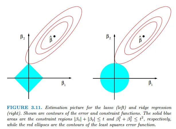
Figure 2: Illustration of L1 and L2 regularization (ESL: page 71)

I had a really hard time understanding this figure until I came across this wonderful blog by explained.ai. I highly recommend you to look into that and various other blogs from the same author available at the site as well. They are really much more intuitive and well explained.

Let's look at the following two diagrams from the above-mentioned blogs:

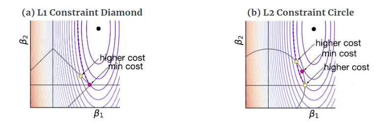
Figure 3: Remember that elliptical curves here are the curves for unconstrained cost function i.e. without any addition of L1 or L2 norms of the coefficients. The black dot at the center of the elliptical curve is the point where the value of cost function is 0 and as we move away from that black dot, its value increases, so higher cost curves are farther from the black dot (Source: explained.ai).

We see that the minimum cost in the case of the L1 is given by the purple dot at the diamond tip. As we move on the edge of the diamond, we find ourselves to be moving away from the black dot and hence there is a higher cost associated with it, for example, look at the yellow dot on the edge of the diamond. Hence in the case of L1 or LASSO regression, it is more likely to find the optimal parameter values at the tip of the diamond.

In contrast to this, let's look at the case of Ridge regression, i.e the L2 constrained circle; we see that the optimal value of parameters is not on the axis since we get the minimum cost at the purple dot, which is away from the axis. To be more clear, let's look at another figure from the same blog:

Figure 4: Zoomed in figure showing the optimal parameters for L1 and L2 regression at the purple point. Moving away from the L1 diamond point immediately increases loss, but L2 can move a little bit upwards before moving leftward away from the loss function minimum. (Source: explained.ai)

Intuition 4: Probabilistic Interpretation of L1 and L2

For this part, I assume that you know some basics of the Bayes Theorem. I will skip a lot of details here. For more details, you can look into the answers to this cross-validated question and this wonderful blog by Brian Keng.

Maximum log-likelihood estimate for a linear regression model can be given by:

$$\hat{\beta}_{MLE} = \arg\max_{\beta} \log P(y|X, \beta) = \arg\min_{\beta} \sum_{i=1}^{n}(y_i - \beta^T x_i)^2$$

We simply choose that β for which mean squared error between the observed value $y$ and predicted value $\hat{y}$ is minimum. With a simple modification to the above expression, the maximum log-likelihood estimate for L1 and L2 regression can be written as follows:

$$\hat{\beta}_{L2} = \arg\min_{\beta} \sum_{i=1}^{n}(y_i - \beta^T x_i)^2 + \lambda ||\beta||_2^2$$ $$\hat{\beta}_{L1} = \arg\min_{\beta} \sum_{i=1}^{n}(y_i - \beta^T x_i)^2 + \lambda ||\beta||_1$$

Likelihood estimate for ordinary linear regression can also be given by following (when we do not consider log) equation:

$$P(y|X, \beta) = \prod_{i=1}^{n} \frac{1}{\sqrt{2\pi\sigma^2}} \exp\left(-\frac{(y_i - \beta^T x_i)^2}{2\sigma^2}\right)$$

From Bayes Theorem we know that the posterior, is defined as follows:

$$P(\beta|y) = \frac{P(y|\beta) \cdot P(\beta)}{P(y)}$$

In case of Bayesian methods we are primarily concerned about the Posterior, i.e. the probability distribution of parameter β given the observed data y in contrast to the classical methods where we try to find the best parameters to maximize the likelihood i.e. the probability of observing data(y) given different value of parameters.

Priors are simply some additional previous information about β before coming across the data y.

The Maximum A Posteriori Probability Estimate (MAP)

In this case, we will try to maximize the $P(\beta|y)$, i.e. the posterior probability. MAP is closely related to the MLE, but also includes prior distribution, therefore it acts as a regularization of MLE.

$$\hat{\beta}_{MAP} = \arg\max_{\beta} P(\beta|y) = \arg\max_{\beta} P(y|\beta) \cdot P(\beta)$$

L2 Regularization and Gaussian Prior

Consider a zero-mean normally distributed prior on each $\beta_i$ value, all with identical variance $\tau^2$:

$$P(\beta_i) = \frac{1}{\sqrt{2\pi\tau^2}} \exp\left(-\frac{\beta_i^2}{2\tau^2}\right)$$

From the likelihood equation and the MAP estimate equation, we have:

$$\hat{\beta}_{MAP} = \arg\max_{\beta} \prod_{i=1}^{n} \frac{1}{\sqrt{2\pi\sigma^2}} \exp\left(-\frac{(y_i - \beta^T x_i)^2}{2\sigma^2}\right) \cdot \prod_{j=1}^{p} \frac{1}{\sqrt{2\pi\tau^2}} \exp\left(-\frac{\beta_j^2}{2\tau^2}\right)$$ $$= \arg\min_{\beta} \sum_{i=1}^{n}(y_i - \beta^T x_i)^2 + \frac{\sigma^2}{\tau^2} ||\beta||_2^2$$

The connection: Thus, we see that the MAP estimate of Linear Regression coefficients with Gaussian priors gives us L2 or Ridge Regression. Note that $\lambda = \sigma^2/\tau^2$ in the above equations.

L1 Regularization and Laplacian Prior

The probability distribution function for Laplace distribution is given by the following equation:

$$P(\beta_i) = \frac{1}{2b} \exp\left(-\frac{|\beta_i|}{b}\right)$$

Considering the zero mean Laplacian priors on all the coefficients as we did in the previous section, we have:

$$\hat{\beta}_{MAP} = \arg\max_{\beta} \prod_{i=1}^{n} \frac{1}{\sqrt{2\pi\sigma^2}} \exp\left(-\frac{(y_i - \beta^T x_i)^2}{2\sigma^2}\right) \cdot \prod_{j=1}^{p} \frac{1}{2b} \exp\left(-\frac{|\beta_j|}{b}\right)$$ $$= \arg\min_{\beta} \sum_{i=1}^{n}(y_i - \beta^T x_i)^2 + \frac{\sigma^2}{b} ||\beta||_1$$

Similarly: Again, we see that MAP of Linear Regression coefficients with Laplacian priors gives us L1 or Lasso Regression.

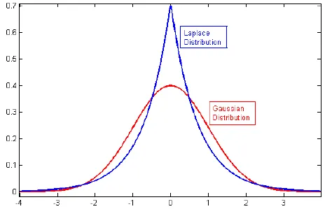
Figure 5: Laplace and Gaussian Distribution (Source: Cross Validated)

Look at the above graph for the Gaussian and Laplace distribution. As we discussed earlier that L1 or LASSO regression can be viewed as putting Laplace priors on the weights. Since the Laplace distribution is more concentrated around zero, our weight is more likely to be zero in the case of L1 or LASSO regularization.

Summary

L1 or LASSO (Least Absolute Shrinkage and Selection Operator) Regularization supports both variable selection and regularization simultaneously.
Both L1 and L2 regularization problems can be solved using the Lagrangian method of constrained optimization.
The lasso penalty will force some of the coefficients quickly to zero. This means that variables are removed from the model, hence the sparsity.
Ridge regression will more or less compress the coefficients to become smaller. This does not necessarily result in 0 coefficients and the removal of variables.